Airbus Anomaly Detection Project

Dedication: First of all, I would like to dedicate this work to Louis Charles BREGUET, designer, builder, pioneer and inventor of modern helicopter.
</img>
Data Challenge - Anomaly Detection
This is a university project in the form of a data challenge that I did during my data science degree at Télécom Paris. This readme summarizes my progress throughout the analysis. For the exact progress, see the notebook file.
Context
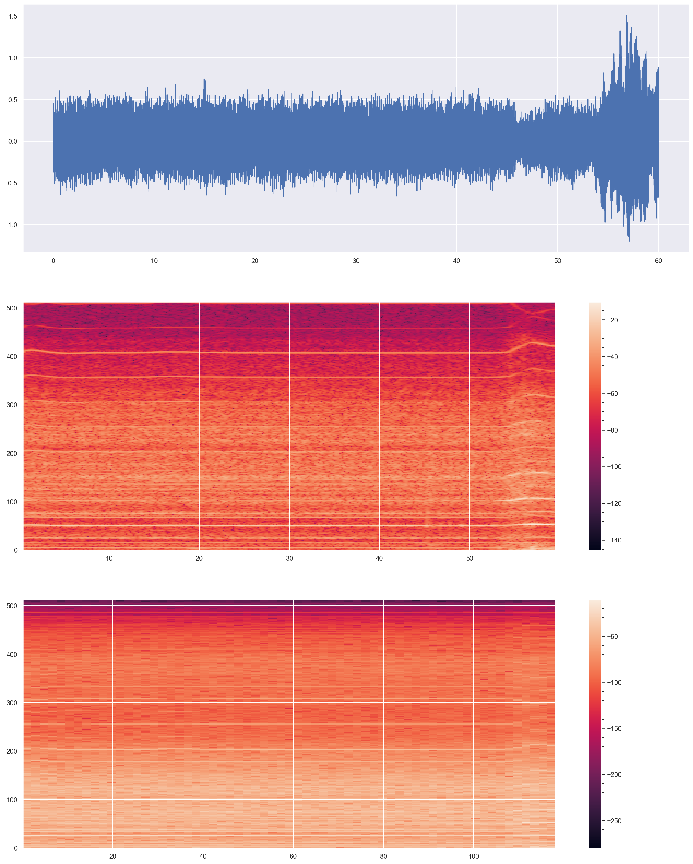
The data set is provided by Airbus and consists of the measures of the accelerometer of helicopters during 1 minute at frequency 1024 Hertz, which yields time series measured at in total 60 * 1024 = 61440 equidistant time points.
Data
Training data
The training set consists of one file, airbus_train.csv.
File airbus_train.csv contains one observation per row, each observation having 61440 entries, measures with equivalent time distance of 1 / 1024 seconds.
There are in total 1677 training observations.
Test data
The training set consists of one file, airbus_test.csv, which has the same structure as file airbus_train.csv.
There are in total 2511 test observations.
Introduction
-
What can be the anormalies?
- What are the possible approaches?
- Raw signal time series observation
- Time Series Clustering
- Similarity
-
DTW (Dynamic Time Warping)
- Periodogram-based distance
- First order/seconde order derivative and other feature engenieering
- Build fonctionnal space
- Interpolation - Spline
- 1st , 2nd order derivative
Some physics before start
What can be the anormalies?
Aircrafte Flutter
Flutter is a dynamic instability of an elastic structure in a fluid flow, caused by positive feedback between the body’s deflection and the force exerted by the fluid flow. In a linear system, “flutter point” is the point at which the structure is undergoing simple harmonic motion—zero net damping—and so any further decrease in net damping will result in a self-oscillation and eventual failure. “Net damping” can be understood as the sum of the structure’s natural positive damping and the negative damping of the aerodynamic force. Flutter can be classified into two types: hard flutter, in which the net damping decreases very suddenly, very close to the flutter point; and soft flutter, in which the net damping decreases gradually. https://www.youtube.com/watch?v=qpJBvQXQC2M&t=59s
https://www.youtube.com/watch?v=MEhVk57ydhw
https://www.youtube.com/watch?v=0FeXjhUEXlc
What are the possible approaches?
Raw signal time series
Similarity
The objective of time series comparison methods is to produce a distance metric between two input time series. The similarity or dissimilarity of two-time series is typically calculated by converting the data into vectors and calculating the Euclidean distance between those points in vector space.
DTW (Dynamic Time Warping)
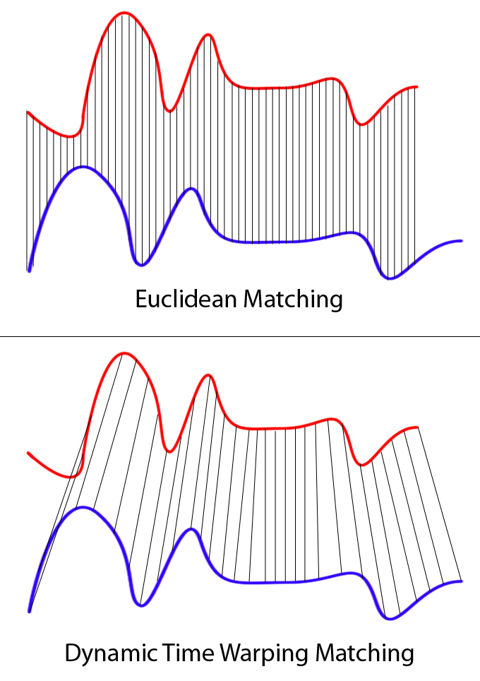
In time series analysis, dynamic time warping (DTW) is one of the algorithms for measuring similarity between two temporal sequences, which may vary in speed. For instance, similarities in walking could be detected using DTW, even if one person was walking faster than the other, or if there were accelerations and decelerations during the course of an observation.
 </img>
Clearly these two series follow the same pattern, but the blue curve is longer than the red. If we apply the one-to-one match, shown in the top, the mapping is not perfectly synced up and the tail of the blue curve is being left out. DTW overcomes the issue by developing a one-to-many match so that the troughs and peaks with the same pattern are perfectly matched, and there is no left out for both curves(shown in the bottom top).
Periodogram-based distance
 </img>
Build fonctionnal space
The Nyquist–Shannon sampling theorem is a theorem in the field of digital signal processing which serves as a fundamental bridge between continuous-time signals and discrete-time signals. It establishes a sufficient condition for a sample rate that permits a discrete sequence of samples to capture all the information from a continuous-time signal of finite bandwidth.
If a function ${\displaystyle }x(t)$ contains no frequencies higher than B hertz, it is completely determined by giving its ordinates at a series of points spaced ${\displaystyle }{\displaystyle 1/(2B)}$ seconds apart.
A sufficient sample-rate is therefore anything larger than ${\displaystyle }2B$ samples per second. Equivalently, for a given sample rate ${\displaystyle }f_{s}$, perfect reconstruction is guaranteed possible for a bandlimit ${\displaystyle }{\displaystyle B<f_{s}/2}$.
Interpolation - Spline
In mathematics, a spline is a special function defined piecewise by polynomials. In interpolating problems, spline interpolation is often preferred to polynomial interpolation because it yields similar results, even when using low degree polynomials, while avoiding Runge’s phenomenon for higher degrees.
2. Frequency Domaine approach with 2 D and 3 D STFT Matrix
Frequency Domaine
Frequency domain refers to the analysis of mathematical functions or signals with respect to frequency, rather than time. Put simply, a time-domain graph shows how a signal changes over time, whereas a frequency-domain graph shows how much of the signal lies within each given frequency band over a range of frequencies.
Perodogram
 </img>
FFT Fast Fourier Transformation
The DTFT, X(e jΩ), is periodic. One period extends from f = 0 to fs, where fs is the sampling frequency.
The FFT contains information between 0 and fs, however, we know that the sampling frequency 5 must be at least twice the highest frequency component. Therefore, the signal’s spectrum should be entirly below fs 2 , the Nyquist frequency.
 </img>
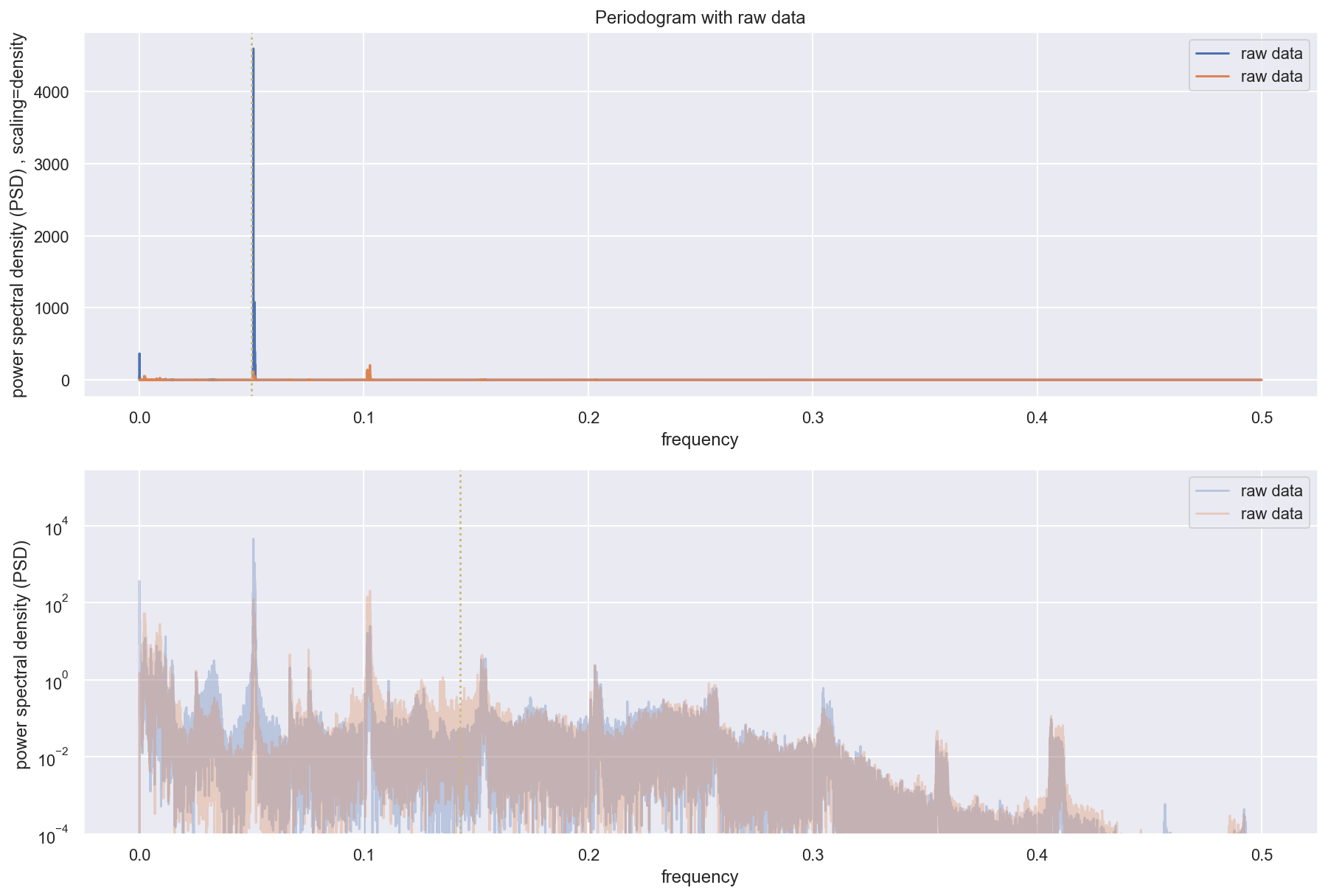
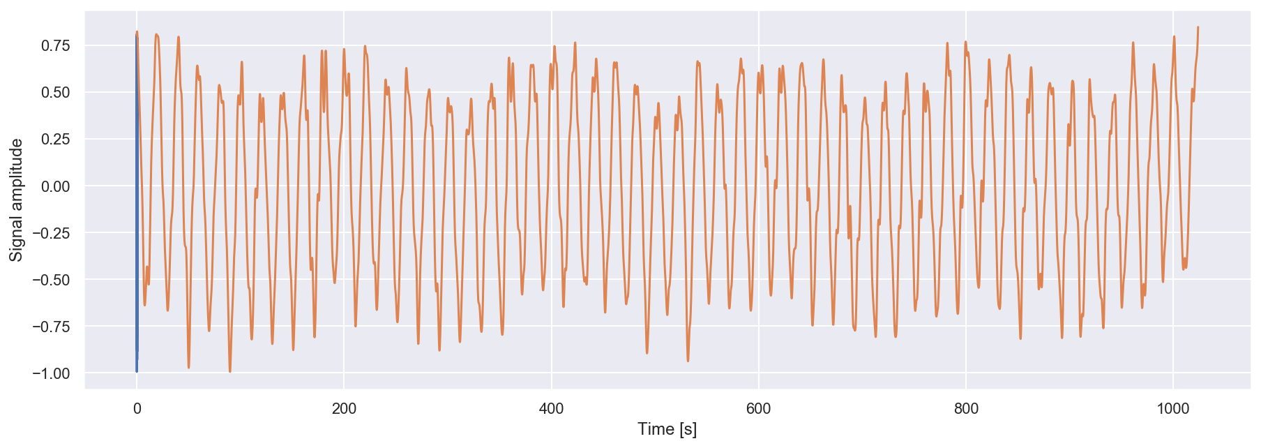
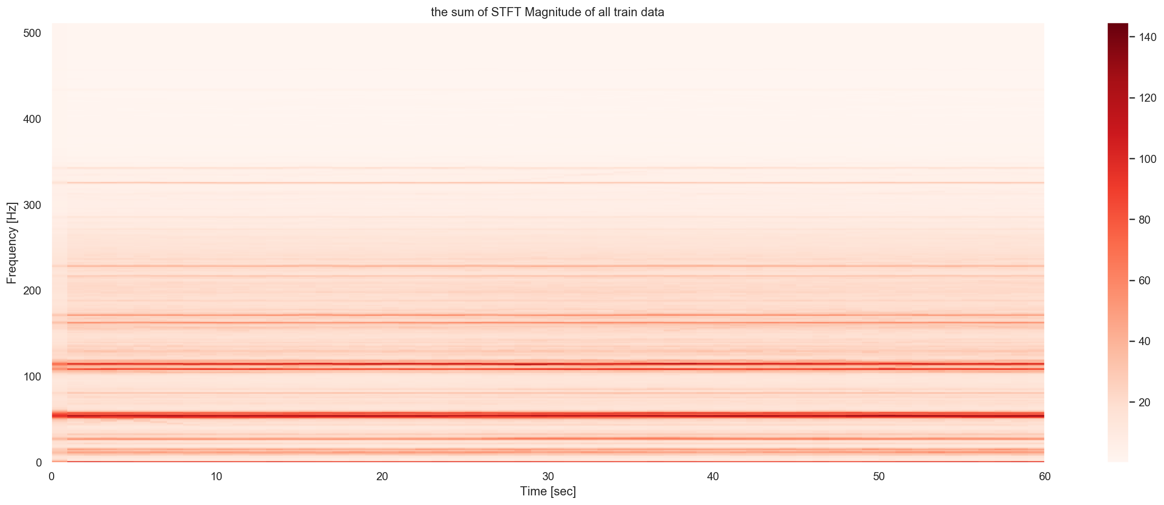
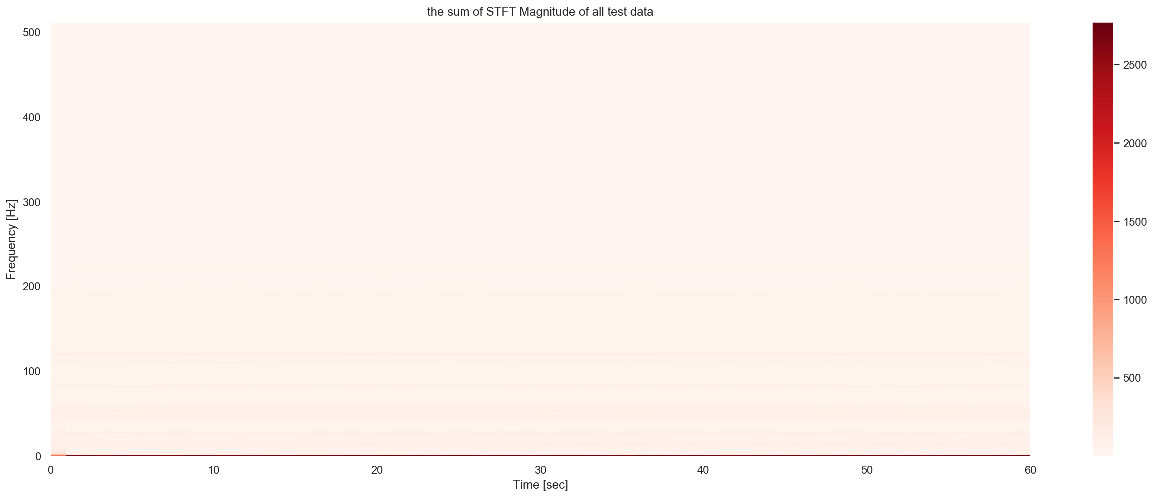
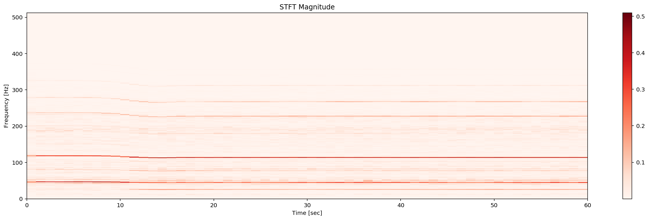
I observe the great difference of global patern of train and test dataset, in the test dataset, a lot of samples are concentrated on 0Hz frenquency. While in the train dataset we can see a very strong density around 50Hz and 100Hz, and their multiples. This corresponde an hypothese of self-exciting ocillation anormaly.
 </img>
 </img>
3. Dimension reduction
As the datasets are large, some detection algorithms would require to reduce the dataset first. This can be done using adapted dimension reduction methods.
PCA
The PCA allows us to reduce the dimensions of both datasets into components that best explain the variance. The graph below shows that the first 20 components seem to explain most of the variance.

We can thus perform our analysis on the first 20 components given by the PCA.
Autoencoder
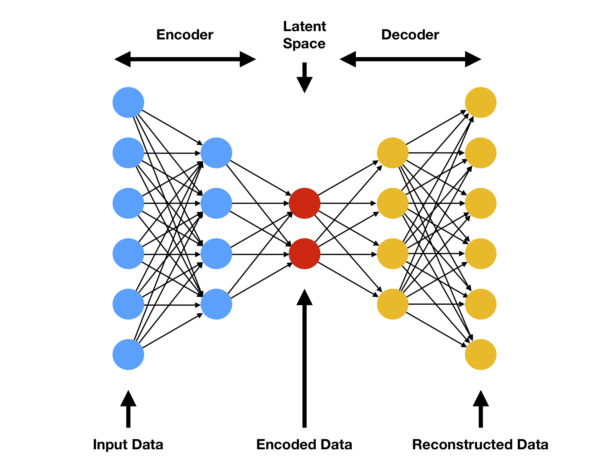
Autoencoder is a more recent algorithm that can be used to perform dimension reduction. It is based on neural networks and can find complex separation functions (whereas PCA is for linear separation only).
 </img>
In the case of a dimension reduction, only the bottleneck (latent space) is relevant for us.
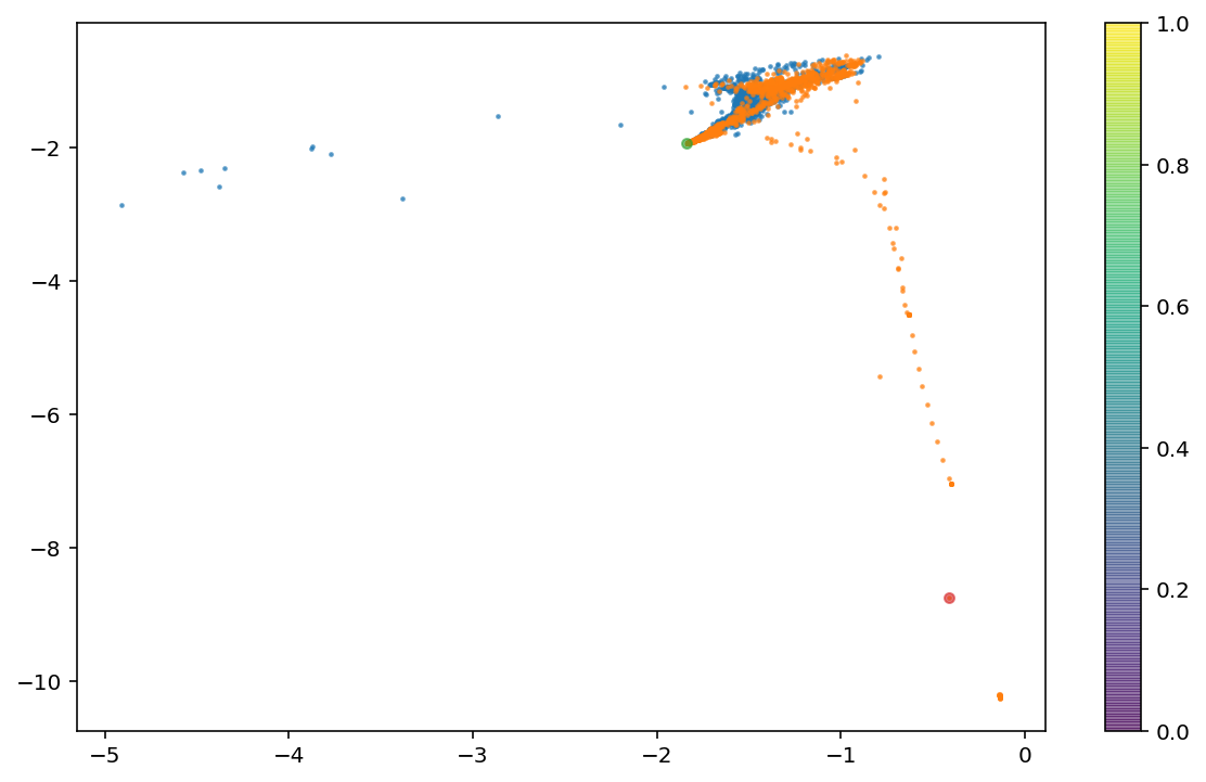
VAE latent space visualization
 </img>
VAE Reconstruction error
 </img>
Surprisingly, PCA gave better results when combined with detection algorithms.
4. Raw Signal Time Series Approach
4.1 LSTM 4.2 LOF + PCA 4.3 Kernel PCA 4.4 OneClassSVM 4.5 Isolation Forest Raw data 4.6 LOF + PCA + Derivatives 4.7 LOF interpolated data 4.8 Isolation Forest Interpolation / 1st order derivative 4.9 Autoencoder with data +der1+der2 4.10 VAE data+der1+der2 4.11 LOF - 1st order derivative and 2nd order derivative 5 Data Augementation
5. Detection algorithms
In order to detect outliers, plenty of algorithms are already implemented and quite easy to use.
Autoencoder
Autoencoders can be used to learn about a distribution and reconstruct some data. The method consists of learning on the train set and scoring on the test set using the following loss function:
 </img>
Observations associated with a higher loss will be more likely to be outliers since they are likely to be very different from the train set.
Isolation forests
Isolation forests are quite intuitive to detect outliers. In short, they allow to isolate abnormal data that have significantly different attributes.
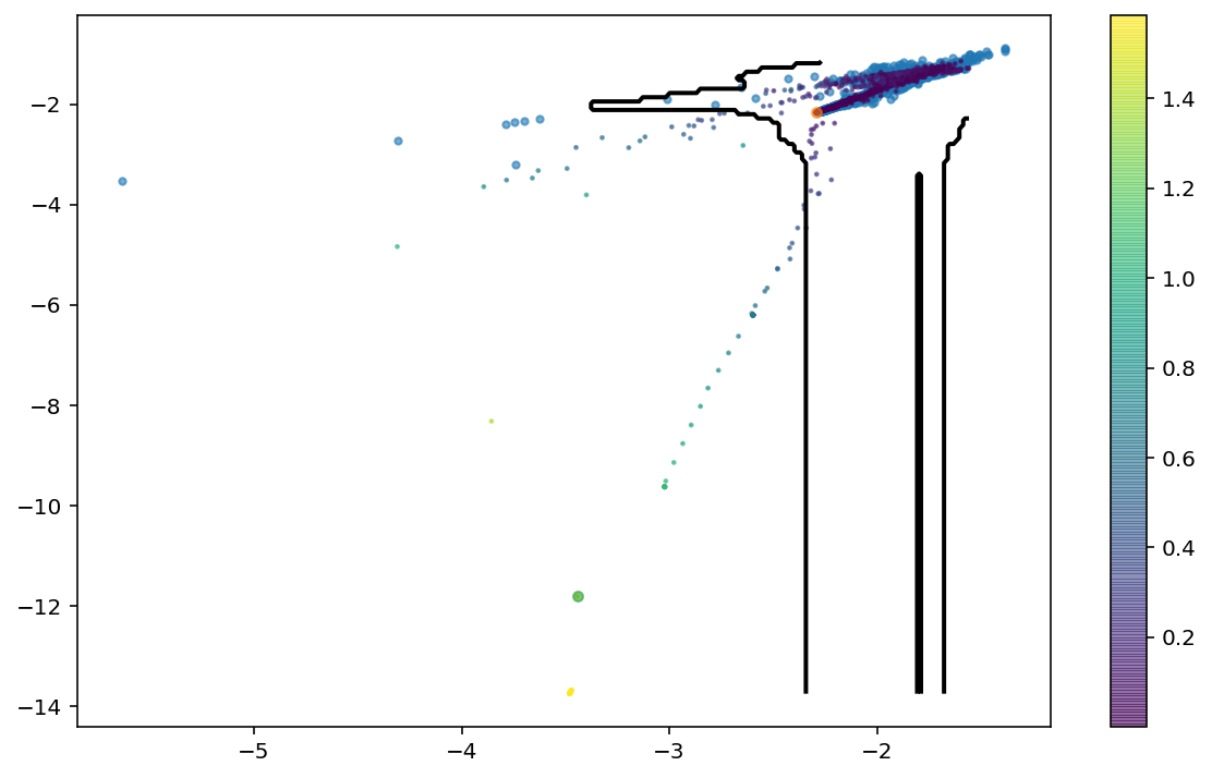
This method gave first satisfactory results when combined with PCA with 20 components.
 </img>
OneClassSVM
 </img>
Local Outlier Factor
Local Outlier Factor is a quite simple detection algorithm that performed really well for this problem. It aims at comparing local densities of test observations with train observations.
Local densities are based on reachability-distance defined as such:
 </img>
The  </img> is the distance between an object and its kth nearest neighbor.
The reachability-distance tells us how far is a point starting from its neighbors.
The distance metric I used is simply the euclidean distance. One of the main advantage of using such an easy metric is that I could easily introduce binary variables when doing feature engineering.
Stacking
I tried to run several models and then to stack their scores but the results were not satisfactory.
6. Feature engineering
Finally, the statistical feature engineering seems to be the best for this project.